Detect data anomalies

---

Caution: Dataplex Explore is deprecated. Support for Explore ends on June 30, 2025. We recommend transitioning your assets to BigQuery Studio for a streamlined data exploration experience across all of Google Cloud analytics tools. See Migrate from Explore to BigQuery Studio.

This document describes how to use Dataplex Explore to detect anomalies in a retail transaction dataset.

The data exploration workbench, or Explore, allows data analysts to interactively query and explore large datasets in real time. Explore helps you gain insights from your data, and lets you query data stored in Cloud Storage and BigQuery. Explore uses a serverless Spark platform, so you don't need to manage and scale the underlying infrastructure.

Objectives

This tutorial shows you how to complete the following tasks:

• Use Explore's Spark SQL workbench to write and execute Spark SQL queries.
• Use a JupyterLab notebook to view the results.
• Schedule your notebook for recurring execution, allowing you to monitor your data for anomalies.

Costs

In this document, you use the following billable components of Google Cloud:

• Dataplex
• Cloud Storage

To generate a cost estimate based on your projected usage, use the pricing calculator. New Google Cloud users might be eligible for a free trial.

When you finish the tasks that are described in this document, you can avoid continued billing by deleting the resources that you created. For more information, see Clean up.

Before you begin

1. Sign in to your Google Cloud account. If you're new to Google Cloud, create an account to evaluate how our products perform in real-world scenarios. New customers also get $300 in free credits to run, test, and deploy workloads.
2. Install the Google Cloud CLI.

3. To initialize the gcloud CLI, run the following command:

   gcloud init

4. Create or select a Google Cloud project.

   Note: If you don't plan to keep the resources that you create in this procedure, create a project instead of selecting an existing project. After you finish these steps, you can delete the project, removing all resources associated with the project.

   • Create a Google Cloud project:

     gcloud projects create PROJECT_ID

     Replace PROJECT_ID with a name for the Google Cloud project you are creating.

   • Select the Google Cloud project that you created:

     gcloud config set project PROJECT_ID

     Replace PROJECT_ID with your Google Cloud project name.

5. Make sure that billing is enabled for your Google Cloud project.

6. Install the Google Cloud CLI.

7. To initialize the gcloud CLI, run the following command:

   gcloud init

8. Create or select a Google Cloud project.

   Note: If you don't plan to keep the resources that you create in this procedure, create a project instead of selecting an existing project. After you finish these steps, you can delete the project, removing all resources associated with the project.

   • Create a Google Cloud project:

     gcloud projects create PROJECT_ID

     Replace PROJECT_ID with a name for the Google Cloud project you are creating.

   • Select the Google Cloud project that you created:

     gcloud config set project PROJECT_ID

     Replace PROJECT_ID with your Google Cloud project name.

9. Make sure that billing is enabled for your Google Cloud project.

Note: Explore is available in the us-central1 and europe-west2 regions only. Make sure that all your data sources (Cloud Storage buckets and BigQuery tables) reside in the same region. Learn more.

Prepare the data for exploration

1. Download the Parquet file, retail_offline_sales_march.

   Download the Parquet file

2. Create a Cloud Storage bucket called offlinesales_curated as follows:

   1. In the Google Cloud console, go to the Cloud Storage Buckets page.

      Go to Buckets page

   2. Click Create bucket.
   3. On the Create a bucket page, enter your bucket information. To go to the next step, click Continue.
      • For Name your bucket, enter a name that meets the bucket naming requirements.
      • For Choose where to store your data, do the following:
        • Select a Location type option.
        • Select a Location option.
      • For Choose a default storage class for your data, select a storage class.
      • For Choose how to control access to objects, select an Access control option.
      • For Advanced settings (optional), specify an encryption method, a retention policy, or bucket labels.
   4. Click Create.

3. Upload the offlinesales_march_parquet file you downloaded to the offlinesales_curated Cloud Storage bucket you created, by following the steps in Upload object from a filesystem.

4. Create a Dataplex lake and name it operations, by following the steps in Create a lake.

5. In the operations lake, add a zone and name it procurement, by following the steps in Add a zone.

6. In the procurement zone, add the offlinesales_curated Cloud Storage bucket you created as an asset, by following the steps in Add an asset.

Select the table to explore

1. In the Google Cloud console, go to the Dataplex Explore page.

2. In the Lake field, select the operations lake.

3. Click the operations lake.

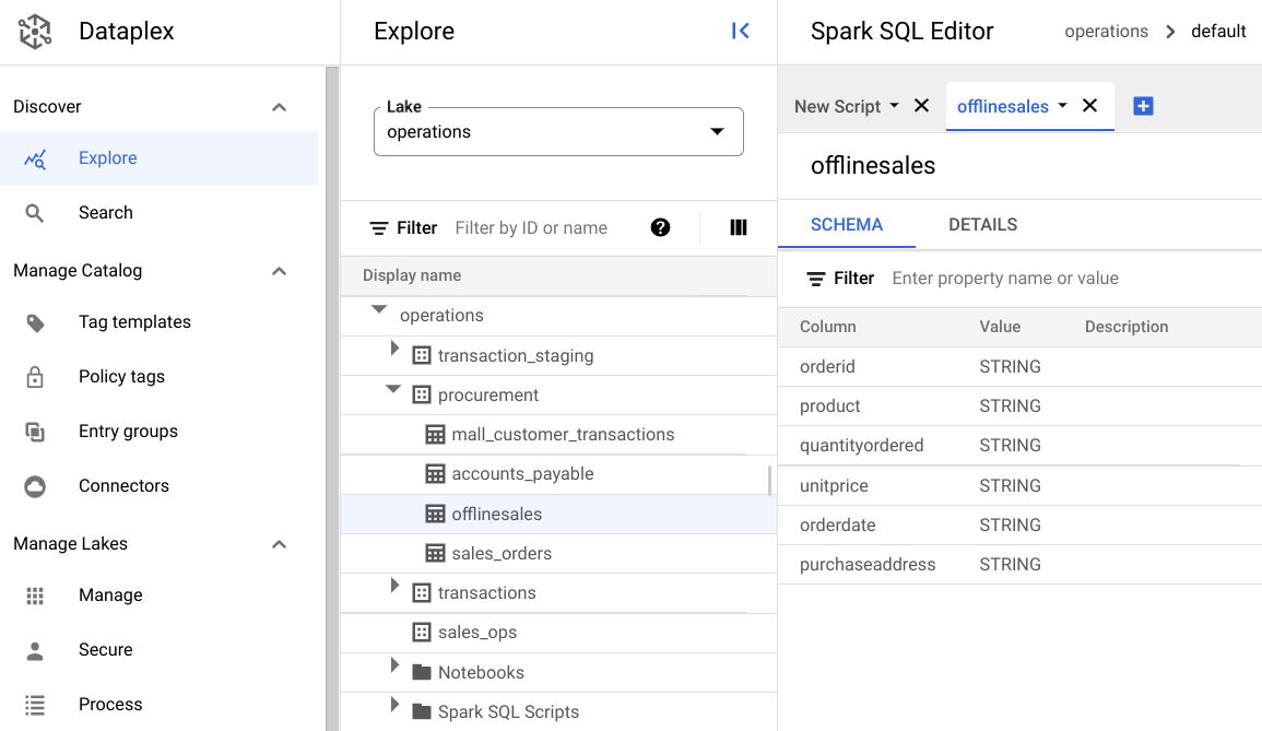
4. Navigate to the procurement zone and click the table to explore its metadata.

   In the following image, the selected procurement zone has a table called Offline, which has the metadata: orderid, product, quantityordered, unitprice, orderdate, and purchaseaddress.

   

5. In the Spark SQL Editor, click Add. A Spark SQL script appears.

6. Optional: Open the script in split tab view to see the metadata and the new script side-by-side. Click More in the new script tab and select Split tab to the right or Split tab to the left.

Explore the data

An environment provides serverless compute resources for your Spark SQL queries and notebooks to run within a lake. Before you write Spark SQL queries, create an environment in which to run your queries.

Explore your data using the following SparkSQL queries. In the SparkSQL Editor, enter the query into the New Script pane.

Sample 10 rows of the table

1. Enter the following query:

   select * from procurement.offlinesales where orderid != 'orderid' limit 10;
   

2. Click Run.

Get the total number of transactions in the dataset

1. Enter the following query:

   select count(*) from procurement.offlinesales where orderid!='orderid';
   

2. Click Run.

Find the number of different product types in the dataset

1. Enter the following query:

   select count(distinct product) from procurement.offlinesales where orderid!='orderid';
   

2. Click Run.

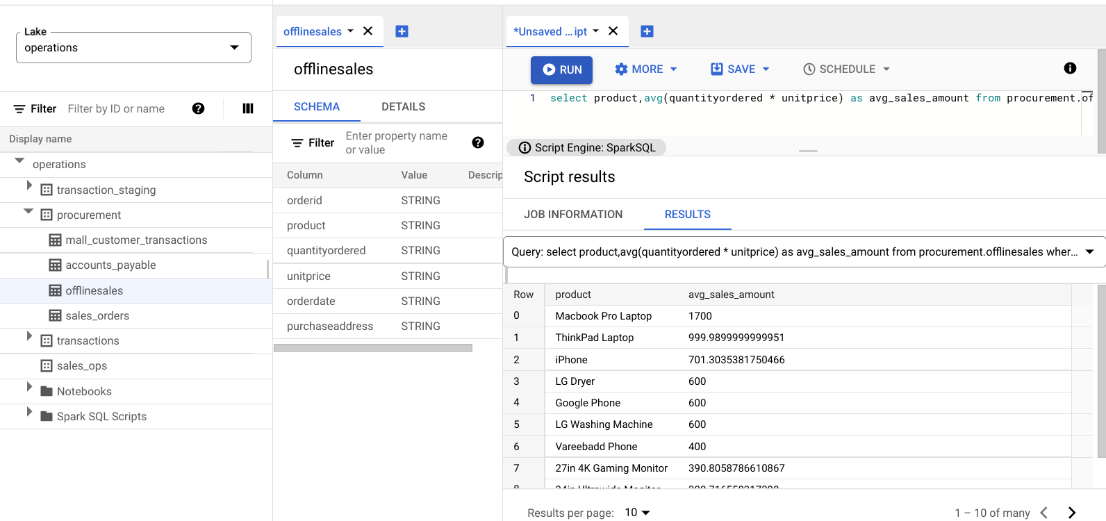
Find the products that have a large transaction value

Get a sense of which products have a large transaction value by breaking down the sales by product type and average selling price.

1. Enter the following query:

   select product,avg(quantityordered * unitprice) as avg_sales_amount from procurement.offlinesales where orderid!='orderid' group by product order by avg_sales_amount desc;
   

2. Click Run.

The following image displays a Results pane that uses a column called product to identify the sales items with large transaction values, shown in the column called avg_sales_amount.

Detect anomalies using coefficient of variation

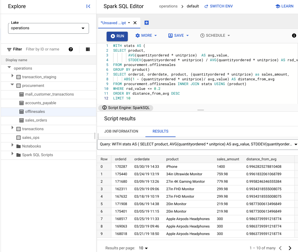
The last query showed that laptops have a high average transaction amount. The following query shows how to detect laptop transactions that aren't anomalous in the dataset.

The following query uses the metric "coefficient of variation", rsd_value, to find transactions that are not unusual, where the spread of values is low compared to the average value. A lower coefficient of variation indicates fewer anomalies.

1. Enter the following query:

   WITH stats AS (
   SELECT product,
         AVG(quantityordered * unitprice)  AS avg_value,
         STDDEV(quantityordered * unitprice) / AVG(quantityordered * unitprice) AS rsd_value
   FROM procurement.offlinesales
   GROUP BY product)
   SELECT orderid, orderdate, product, (quantityordered * unitprice) as sales_amount,
       ABS(1 - (quantityordered * unitprice)/ avg_value) AS distance_from_avg
   FROM procurement.offlinesales INNER JOIN stats USING (product)
   WHERE rsd_value <= 0.2
   ORDER BY distance_from_avg DESC
   LIMIT 10
   

2. Click Run.

3. See the script results.

   In the following image, a Results pane uses a column called product to identify the sales items with transaction values that are within the variation coefficient of 0.2.

   

Visualize anomalies using a JupyterLab notebook

Build an ML model to detect and visualize anomalies at scale.

1. Create a notebook.

2. Open the notebook in a separate tab and wait for it to load. The session in which you executed the Spark SQL queries continues.

3. Import the necessary packages and connect to the BigQuery external table that contains the transactions data. Run the following code:

   from google.cloud import bigquery
   from google.api_core.client_options import ClientOptions
   import os
   import warnings
   warnings.filterwarnings('ignore')
   import pandas as pd
   
   project = os.environ['GOOGLE_CLOUD_PROJECT']
   options = ClientOptions(quota_project_id=project)
   client = bigquery.Client(client_options=options)
   client = bigquery.Client()
   
   #Load data into DataFrame
   
   sql = '''select * from procurement.offlinesales limit 100;'''
   df = client.query(sql).to_dataframe()
   

4. Run the isolation forest algorithm to discover the anomalies in the dataset:

   to_model_columns = df.columns[2:4]
   from sklearn.ensemble import IsolationForest
   clf=IsolationForest(n_estimators=100, max_samples='auto', contamination=float(.12), \
                           max_features=1.0, bootstrap=False, n_jobs=-1, random_state=42, verbose=0)
   clf.fit(df[to_model_columns])
   pred = clf.predict(df[to_model_columns])
   df['anomaly']=pred
   outliers=df.loc[df['anomaly']==-1]
   outlier_index=list(outliers.index)
   #print(outlier_index)
   #Find the number of anomalies and normal points here points classified -1 are anomalous
   print(df['anomaly'].value_counts())
   

5. Plot the predicted anomalies using a Matplotlib visualization:

   import numpy as np
   from sklearn.decomposition import PCA
   pca = PCA(2)
   pca.fit(df[to_model_columns])
   res=pd.DataFrame(pca.transform(df[to_model_columns]))
   Z = np.array(res)
   plt.title("IsolationForest")
   plt.contourf( Z, cmap=plt.cm.Blues_r)
   b1 = plt.scatter(res[0], res[1], c='green',
                   s=20,label="normal points")
   b1 =plt.scatter(res.iloc[outlier_index,0],res.iloc[outlier_index,1], c='green',s=20,  edgecolor="red",label="predicted outliers")
   plt.legend(loc="upper right")
   plt.show()
   

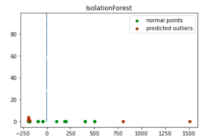
This image shows the transaction data with the anomalies highlighted in red.

Schedule the notebook

Explore lets you schedule a notebook to run periodically. Follow the steps to schedule the Jupyter Notebook you created.

Dataplex creates a scheduling task to run your notebook periodically. To monitor the task progress, click View schedules.

Share or export the notebook

Explore lets you share a notebook with others in your organization using IAM permissions.

Review the roles. Grant or revoke Dataplex Viewer (roles/dataplex.viewer), Dataplex Editor (roles/dataplex.editor), and Dataplex Administrator (roles/dataplex.admin) roles to users for this notebook. After you share a notebook, users with the viewer or editor roles at the lake level can navigate to the lake and work on the shared notebook.

To share or export a notebook, see Share a notebook or Export a notebook.

Clean up

To avoid incurring charges to your Google Cloud account for the resources used in this tutorial, either delete the project that contains the resources, or keep the project and delete the individual resources.

Delete the project

Caution: Deleting a project has the following effects:

• Everything in the project is deleted. If you used an existing project for the tasks in this document, when you delete it, you also delete any other work you've done in the project.
• Custom project IDs are lost. When you created this project, you might have created a custom project ID that you want to use in the future. To preserve the URLs that use the project ID, such as an appspot.com URL, delete selected resources inside the project instead of deleting the whole project.

If you plan to explore multiple architectures, tutorials, or quickstarts, reusing projects can help you avoid exceeding project quota limits.

Delete a Google Cloud project:

gcloud projects delete PROJECT_ID

Delete individual resources

1. Delete the bucket:

   gcloud storage buckets delete BUCKET_NAME

   Important: Your bucket must be empty before you can delete it.
2. Delete the instance:

   gcloud compute instances delete INSTANCE_NAME

What's next

• Learn more about Dataplex Explore.
• Schedule scripts and notebooks.