Pipelines are executed on clusters of machines. They achieve high throughput by splitting up the work that needs to be done, and then running the work in parallel on the multiple executors spread out across the cluster. In general, the greater the number of splits (also called partitions), the faster the pipeline can be run. The level of parallelism in your pipeline is determined by the sources and shuffle stages in the pipeline.
Sources
At the start of each pipeline run, every source in your pipeline calculates what data needs to be read, and how that data can be divided into splits. For example, consider a basic pipeline that reads from Cloud Storage, performs some Wrangler transformations, and then writes back to Cloud Storage.
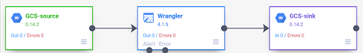
When the pipeline starts, the Cloud Storage source examines the input files and breaks them up into splits based on the file sizes. For example, a single gigabyte file can be broken up into 100 splits, each 10 MB in size. Each executor reads the data for that split, runs the Wrangler transformations, and then writes the output to a part file.

If your pipeline is running slowly, one of the first things to check is whether your sources are creating enough splits to take full advantage of parallelism. For example, some types of compression make plaintext files unsplittable. If you are reading files that have been gzipped, you might notice that your pipeline runs much slower than if you were reading uncompressed files, or files compressed with BZIP (which is splittable). Similarly, if you are using the database source and have configured it to use just a single split, it runs much slower than if you configure it to use more splits.
Shuffles
Certain types of plugins cause data to be shuffled across the cluster. This happens when records being processed by one executor need to be sent to another executor to perform the computation. Shuffles are expensive operations because they involve a lot of I/O. Plugins that cause data to be shuffled all show up in the Analytics section of the Pipeline Studio. These include plugins, such as Group By, Deduplicate, Distinct, and Joiner. For example, suppose a Group By stage is added to the pipeline in the preceding example.
Also suppose the data being read represents purchases made at a grocery store.
Each record contains an item field and a num_purchased field. In the Group
By stage, we configure the pipeline to group records on the item field and
calculate the sum of the num_purchased field.
When the pipeline runs, the input files are split up as described earlier. After that, each record is shuffled across the cluster such that every record with the same item belongs to the same executor.
As illustrated in the preceding example, records for apple purchases were originally spread out across several executors. To perform the aggregation, all of those records needed to be sent across the cluster to the same executor.
Most plugins that require a shuffle let you to specify the number of partitions to use when shuffling the data. This controls how many executors are used to process the shuffled data.
In the preceding example, if the number of partitions is set to 2, each executor calculates aggregates for two items instead of one.
Note that it is possible to decrease the parallelism of your pipeline after that stage. For example, consider the logical view of the pipeline:
If the source divides data across 500 partitions but the Group By shuffles using 200 partitions, the maximum level of parallelism after the Group By drops from 500 to 200. Instead of 500 different part files written to Cloud Storage, you only have 200.
Choosing partitions
If the number of partitions is too low, you won't be using the full capacity of your cluster to parallelize as much work as you can. Setting the partitions too high increases the amount of unnecessary overhead. In general, it is better to use too many partitions than too few. Extra overhead is something to worry about if your pipeline takes a few minutes to run and you are trying to shave off a couple minutes. If your pipeline takes hours to run, overhead is generally not something you need to worry about.
A useful, but overly simplistic, way to determine the number of partitions to
use is to set it to max(cluster CPUs, input records / 500,000). In other
words, take the number of input records and divide by 500,000. If that number is
greater than the number of cluster CPUs, use that for the number of partitions.
Otherwise, use the number of cluster CPUs. For example, if your cluster has
100 CPUs and the shuffle stage is expected to have 100 million input
records, use 200 partitions.
A more complete answer is that shuffles perform best when the intermediate shuffle data for each partition can fit completely in an executor's memory so that nothing needs to be spilled to disk. Spark reserves just under 30% of an executor's memory for holding shuffle data. The exact number is (total memory - 300 MB) * 30%. If we assume each executor is set to use 2 GB memory, that means each partition should hold no more than (2 GB - 300 MB) * 30% = approximately 500 MB of records. If we assume each record compresses down to 1 KB in size, then that means (500 MB / partition) / (1 KB / record) = 500,000 records per partition. If your executors are using more memory, or your records are smaller, you can adjust this number accordingly.
Data skew
Note that in the preceding example, purchases for various items were evenly distributed. That is, there were three purchases each for apples, bananas, carrots, and eggs. Shuffling on an evenly distributed key is the most performant type of shuffle, but many datasets don't have this property. Continuing the grocery store purchase in the preceding example, you would expect to have many more purchases for eggs than for wedding cards. When there are a few shuffle keys that are much more common than other keys, you are dealing with skewed data. Skewed data can perform significantly worse than unskewed data because a disproportionate amount of work is being performed by a small handful of executors. It causes a small subset of partitions to be much larger than all the others.
In this example, there are five times as many egg purchases than card purchases, which means the egg aggregate takes roughly five times longer to compute. It doesn't matter much when dealing with just 10 records, instead of two, but it makes a big difference when dealing with five billion records instead of one billion. When you have data skew, the number of partitions used in a shuffle doesn't have a large impact on pipeline performance.
You can recognize data skew by examining the graph for output records over time. If the stage is outputting records at a much higher pace at the start of the pipeline run and then suddenly slows down, this might mean you have skewed data.
You can also recognize data skew by examining cluster memory usage over time. If your cluster is at capacity for some time, but suddenly has low memory usage for a period of time, this is also a sign that you are dealing with data skew.
Skewed data most significantly impacts performance when a join is being
performed. There are a few techniques that can be used to improve performance
for skewed joins. For more information, see
Parallel processing for JOIN operations.
Adaptive tuning for execution
To adaptively tune execution, specify the range of partitions to use, not the exact partition number. The exact partition number, even if set in pipeline configuration, is ignored when adaptive execution is enabled.
If you are using an ephemeral Dataproc cluster, Cloud Data Fusion sets proper configuration automatically, but for static Dataproc or Hadoop clusters, the next two configuration parameters can be set:
spark.default.parallelism: set it to the total number of vCores available in the cluster. This ensures your cluster isn't underloaded and defines the lower bound for the number of partitions.spark.sql.adaptive.coalescePartitions.initialPartitionNum: set it to 32x of the number of vCores available in the cluster. This defines the upper bound for the number of partitions.Spark.sql.adaptive.enabled: to enable the optimizations, set this value totrue. Dataproc sets it automatically, but if you are using generic Hadoop clusters, you must ensure it's enabled .
These parameters can be set in the engine configuration of a specific pipeline or in the cluster properties of a static Dataproc cluster.
What's next
- Learn about parallel processing for
JOINoperations.